How to Stop Over-Evaluating LLMs using this Simple Statistical Fact
When we evaluate a new LLM checkpoint, the default is usually simple: run the whole benchmark.
That is often reasonable, but for frequent iterations (think frequently updated models, frequent model health check, etc) it can be unnecessarily expensive. In many settings, what we actually need is not "full coverage", but a reliable estimate with controlled uncertainty.
Last year, I was in an "Researchers and Founders" event in San Francisco, and a founder of an AI startup that works mainly on model eval asked me the following question: what is a simple mathematical fact that would significantly improve what we're doing?
I mentioned that simple uncertainty estimates could help significantly make eval more efficient. I'm writing this blog to futher explain this simple result, and how one can make most of it. In this post, I focus on a basic question:
How many benchmark examples do we really need to estimate accuracy well?
1) Subset Evaluation and Why it Works
For many common benchmarks, the metric is accuracy (or exact match), which is just an average of binary outcomes.
For each example , define
Then true benchmark accuracy is which is the average across a hypothetical infinite number of samples. In practice, we only have access to finite number of examples, and subset accuracy on examples is
So this is a standard sample-mean estimation problem, and is a noisy estimate of the true accuracy . Note that , so on average is a "good" estimate of . In statistics language, we call an unbiased estimator of . We can write as follows
which provides a nice interpretation of : the true accuracy , plus an additional estimation error () which is due to finite sample size.
Intuitively, the quality of the estimator could be measured by the magnitude of the error . One possible way to measure this is by considering the variance . It is easy to check in this case that
Now the key property here is boundedness of the sample variance
which implies that the estimation error (measured by the variance) is bounded
In other words, the estimation error (measured by the variance) is bounded by a quantity that is model-and-data-independent! This is the main (theoretical) reason subset evaluation is useful for accuracy metrics: uncertainty scales in a controlled way with .
2) A Practical Rule for Choosing Subset Size
Now suppose we want to benchmark a model on some dataset, and we want to do things efficiently: select the smallest subset size such that our estimated accuracy is guaranteed to be within some range of the true accuracy.
Mathematically, we want something like this
where is the target error tolerance (for example, 0.02 for accuracy) and is confidence.
Using a Gaussian approximation with worst-case variance, a practical sizing rule is
At 95% confidence ():
For , this gives
This is conservative, but operational: instead of evaluating everything by default, we can pick a sample size aligned with a target uncertainty.
3) Application to Evals
Most evaluation is not a one-time event. We repeatedly evaluate during:
- model iteration,
- hyperparameter sweeps,
- ablations,
- regressions after code or data changes.
In these loops, we usually need "decision-grade" certainty, not perfect certainty. A principled subset can reduce evaluation cost while still preserving statistical control.
Figure 1 shows subset eval for Qwen3-4B on Hellaswag. The x-axis is the subset size, and y-axis is the accuracy. I'm using 12 random seeds to obtain the distribution of accuracy scores for each subset size . The gray dashed lines represent the theoretical confidence intervals discussed above (95% confidence) and the blue shaded area represent the range of eval accuracy as we vary the random seed. The theoretical range cover the range of the observed accuracy. The red dashed line reprsents the theoretical prediction that guarantees an estimation error of no more than from the true accuracy , with confidence.
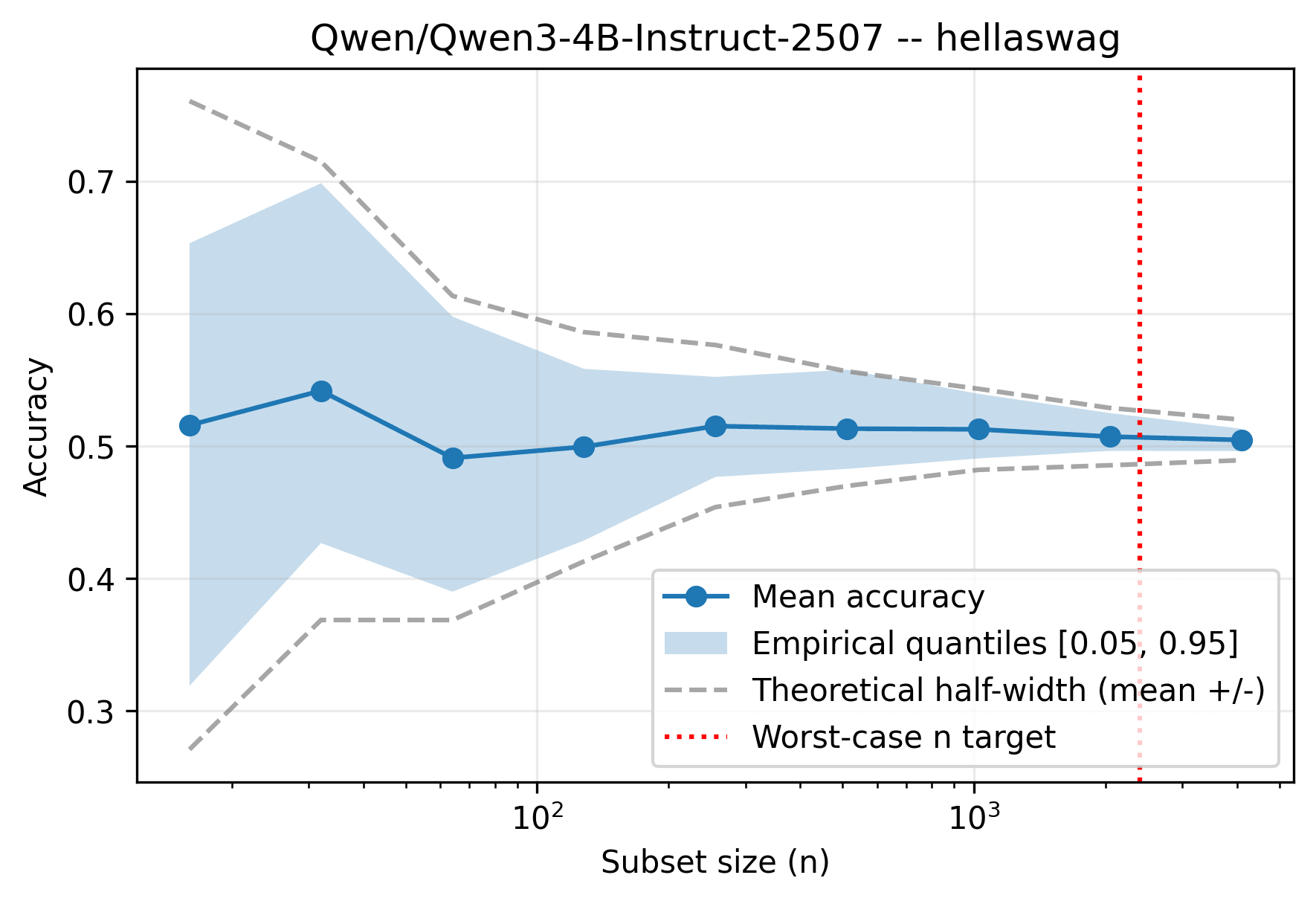
Figure 1: Efficient evaluation pipeline.
4) A Better Bound Means More Efficiency
The bound is worst-case and fully conservative.
If we have prior knowledge that the model is already fairly good, we can tighten it.
For Bernoulli accuracy, we have
If we know , then
so
which is strictly better than .
This translates directly into sample size. Using the same Gaussian sizing logic,
Under the conservative bound, this is proportional to .
Under , it is proportional to at most .
So for the same error tolerance and confidence, you need about
times as many examples, i.e. roughly 16% fewer evaluations.
In repeated eval loops, that gap compounds quickly: better variance bounds give the same statistical reliability at lower cost.
5) Final Remark
Running the full benchmark is not "wrong". But for iterative model development, it is often more useful to choose evaluation size based on target uncertainty rather than habit.
The main gain is not only speed. It is the ability to report a number together with a quantitative level of confidence, which makes evaluation easier to trust and easier to scale.